본 포스트는 패스트캠퍼스 파이썬 기초부터 시작하는 딥러닝 영상인식 바이블 강의를 정리한 글입니다.

올해 상반기가 지나가기 전 딥러닝 공부를 깊게 해보고 싶었다. CNN, RNN, LSTM 등의 이론은 학부생활을 하면서 꽤나 익혔는데, 딥러닝 프레임워크를 사용하여 모델링하는 것은 해보지 않았기에, 프레임워크 중 한 가지 정도는 능숙하게 사용하는 것을 목표로 삼게 되었다. 강의를 따라 keras를 사용할 예정인데, 

keras 문서 를 들어가 사용법을 볼 수 있고, 기본적인 모델링은 문서를 통해 배울 수 있을 것 같다. 

1. 필요 라이브러리 import 

# TensorFlow and tf.keras
import tensorflow as tf 
from tensorflow import keras 
#  Helper libraries 
import numpy as np 
import matplotlib.pyplot as plt 
import math

print(tf.__version__) # tensorflow 버전 확인

tensorflow, keras를 import 해준다.  필자는 google colab 에서 실습을 진행하였고, 글을 쓰는 시점을 기준으로 tf 버전 2.8.0 을 사용한다. 이 밖에 필요한 numpy, matplotlib, math를 import 해 준다. 

2. batch size, epochs, num_classes 정의

# Define Constants 
batch_size = 128 
epochs = 100 
num_classes = 10

batch_size: 데이터를 몇개씩 묶어서 학습할 것인가? -> 128개씩 묶어서 학습하겠다

ephocs: 학습을 반복하는 횟수 -> 100번 학습하겠다

num_classes: 클래스의 개수 -> MNIST는 0~9까지 10개이므로 10

• 60000장의 데이터를 한번에 학습하지 않고 batch size를 설정하는 이유

배치를 나눠서 학습하게되면 모든 데이터가 스트레이트로 쭉 학습되는 것이 아니라, batch size만큼 학습되면서 예측 값이 맞거나 틀린 경우가 각 배치마다 업데이트 되기 때문에 중간중간 가중치가 조절될 수 있으므로 더 좋은 성능을 기대해볼 수 있다.

(실제로 실험해보았더니 batch size를 60000장으로 했을 때 정확도가 0.02정도 낮게 나왔다. (MNIST 데이터 기준) 그리고 batch size가 작아질 수록 학습 속도가 느려진다. 아직 배치사이즈를 조정할 레벨은 아니지만, 배치사이즈에 따라 성능이 달라지는 것을 직접 확인하니 적절한 배치사이즈를 설정해주는 것도 중요한 부분인 것 같아보인다. )

3. MNIST 데이터셋 불러오기

# Download MNIST dataset 
mnist = keras.datasets.mnist
(train_images, train_labels), (test_images, test_labels) = mnist.load_data()

워낙 유명한 MNIST 데이터셋은 keras에서 제공해주므로 따로 다운받을 필요 없이 위와 같은 코드를 작성하여 사용할 수 있다.  

len(train_images), len(test_images)

 (60000, 10000) 

train은 60000장, test는 10000장임을 알 수 있다. 

4. 딥러닝 모델 학습

(1) normailze (0.0 ~ 1.0 사이의 값이 되도록) 

# Normalize the input image so that each pixel value is between 0 to 1 
train_images = train_images / 255.0 
test_images = test_images / 255.0

데이터를 float형으로 만들면서 0.0~1.0 사이로 정규화해준다. 

(2) 딥러닝 모델 정의

# Define the model architecture 
model = keras.Sequential([
                          keras.layers.Flatten(input_shape=(28, 28)),
                          keras.layers.Dense(128, activation=tf.nn.relu),
                          keras.layers.Dense(num_classes, activation='softmax')
])
model.compile(optimizer='adam',
              loss=tf.keras.losses.SparseCategoricalCrossentropy(from_logits=True),
              metrics=['accuracy'])

모델은 keras.Sequential에 층을 하나하나 추가해주는 방식이다. 직관적으로 모델링을 할 수 있다는 장점이 있다. flatten으로 한 장당 2차원 배열 28x28인 이미지를 1차원으로 만들어 준다. 그다음 Dense layer를 사용하고, activation 함수는 relu를 사용한다. 마지막 층에는 클래스의 개수와 softmax 함수를 사용함으로써 예측 결과를 클래스 별 확률로 나오게끔 만들어준다. 

model.complie로 optimizer와 loss함수, metrics (평가지표)를 설정해 준다. 

이제 모델 학습할 모든 준비가 되었다. 

(3) 딥러닝 모델 학습

history = model.fit(train_images, train_labels, epochs=epochs, batch_size=batch_size)

train 데이터셋과 앞서 지정했던 ephocs, batch_size를 설정해 준다. 

5. 딥러닝 모델 평가

(1) loss, accuracy 확인

test_loss, test_acc = model.evaluate(test_images, test_labels)
print("Test Loss: ", test_loss)
print("Test Accuracy: ", test_acc)

 Test Loss: 0.12909765541553497 

 Test Accuracy: 0.98089998960495 

아주 기본적인 딥러닝 모델을 사용하였음에도 불구하고 0.98이라는 높은 정확도가 나왔다. 모든 학습 결과가 이랬으면 좋겠다. 

(2) 필요 함수 정의 

# 1. 원하는 개수만큼 이미지를 보여주는 함수 
def show_sample(images, labels, sample_count=25):
  # Create a square with can fit {sample_count} images
  grid_count = math.ceil(math.ceil(math.sqrt(sample_count)))
  grid_count = min(grid_count, len(images), len(labels))

  plt.figure(figsize=(2*grid_count, 2*grid_count))
  for i in range(sample_count):
    plt.subplot(grid_count, grid_count, i+1)
    plt.xticks([])
    plt.yticks([])
    plt.grid(False)
    plt.imshow(images[i], cmap=plt.cm.gray)
    plt.xlabel(labels[i])
  plt.show()

###################################################################
# 2. 특정 숫자의 이미지를 보여주는 함수 
# Helper function to display specific digit images 
def show_sample_digit(images, labels, digit, sample_count=25):
  # Create a square with can fit {sample_count} images
  grid_count = math.ceil(math.ceil(math.sqrt(sample_count)))
  grid_count = min(grid_count, len(images), len(labels))

  plt.figure(figsize=(2*grid_count, 2*grid_count))
  i = 0 
  digit_count = 0 
  while digit_count < sample_count:
    i += 1 
    if digit == labels[i]: 
      plt.subplot(grid_count, grid_count, digit_count+1)
      plt.xticks([])
      plt.yticks([])
      plt.grid(False)
      plt.imshow(images[i], cmap=plt.cm.gray)
      plt.xlabel(labels[i])
      digit_count += 1 
  plt.show()


###################################################################
# 3.이미지 한개를 크게 보여주는 함수 
def show_digit_image(image):
  # Draw digit image 
  fig = plt.figure()
  ax = fig.add_subplot(1, 1, 1)
  # Major ticks every 20, minor ticks every 5 
  major_ticks = np.arange(0, 29, 5)
  minor_ticks = np.arange(0, 29, 1)
  ax.set_xticks(major_ticks)
  ax.set_xticks(minor_ticks, minor=True)
  ax.set_yticks(major_ticks)
  ax.set_yticks(minor_ticks, minor=True)
  # And a corresponding grid 
  ax.grid(which='both')
  # Or if you want different settings for the grids:
  ax.grid(which='minor', alpha=0.2)
  ax.grid(which='major', alpha=0.5)
  ax.imshow(image, cmap=plt.cm.binary)

  plt.show()

28x28 배열의 이미지를 시각화로 확인해볼 수 있도록 해주는 함수이다. 

위 함수를 사용하여 잠깐 이미지를 확인해 보자. 

• show_sample 함수 사용 (원하는 개수만큼 사진 출력)

show_sample(train_images, ['Label: %s' % label for label in train_labels])

이렇게 원하는 개수 만큼 이미지를 확인해볼 수 있다. 

• show_sample_digit 함수 사용 (특정 숫자에 대한 원하는 개수만큼의 사진 출력)

show_sample_digit(train_images, train_labels, 7)

특정 숫자를 원하는 개수만큼 확인해볼 수 있다. 

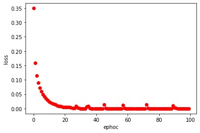
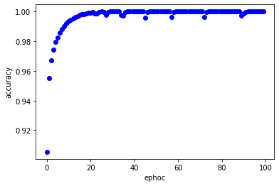
(3) train 데이터셋 학습 시 ephoch에 따른 loss와 accuracy 값 시각화

# Evaluate the model using test dataset. - Show performance 
fig, loss_ax = plt.subplots()
fig, acc_ax = plt.subplots()

loss_ax.plot(history.history['loss'], 'ro')
loss_ax.set_xlabel('ephoc')
loss_ax.set_ylabel('loss')

acc_ax.plot(history.history['accuracy'], 'bo')
acc_ax.set_xlabel('ephoc')
acc_ax.set_ylabel('accuracy')

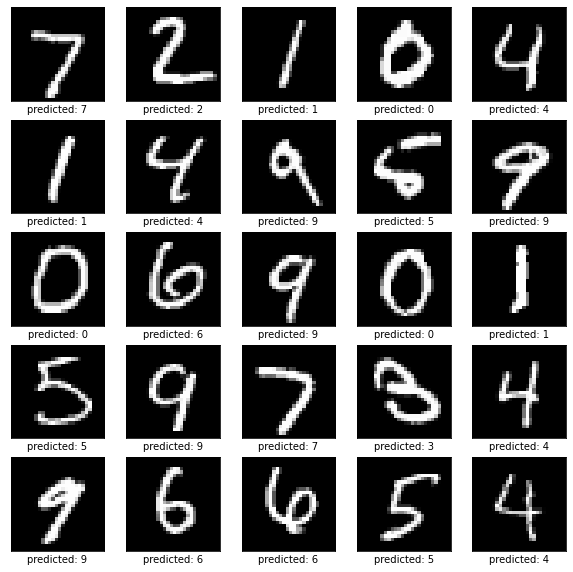
(4) test data의 예측 값과 정답 값 비교해보기

• 실제값: 그림
• 예측값: x label

# Predict the labels of digit images in our test datasets.
predictions = model.predict(test_images)

# Then plot the first 25 test images and their predicted labels.
show_sample(test_images, ['predicted: %s' % np.argmax(result) for result in predictions])

(5) show_digit_image 함수 사용

• 특정 인덱스의 사진과 그때의 예측값을 비교해 봄

Digit = 2005 #@param {type:'slider', min:1, max:10000, step:1}
selected_digit = Digit - 1 

result = predictions[selected_digit]
result_number = np.argmax(result)
print('Number is %2d' % result_number)

show_digit_image(test_images[selected_digit])

#@param을 사용하면 위와 같이 슬라이더가 생긴다. 랜덤으로 슬라이드를 해서 인덱스 값을 지정해 주면,

Number is 7

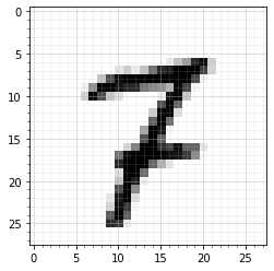
이와 같이 Number is 7 은 예측 값, 이미지는 test 이미지 (정답 값)으로 두개를 비교 확인해볼 수 있다. 

이번 포스트에서 사용한 MNIST데이터셋은 아주 간단한 딥러닝 모델인데도 성능이 좋았다. 

다음 포스팅에서는 이미지 모델학습에 최적화 되어있는 CNN 모델링을 함으로써 MNIST의 성능을 더욱 높여보는 공부를 해 볼 것이다. 

사용 데이터셋 

https://www.data.go.kr/dataset/3035522/fileData.do

현재 이 데이터셋은 폐기 되었다고 나온다. 

위 공공데이터를 사용하여 인프런강의 (공공데이터로 파이썬 데이터 분석) (https://bit.ly/3sISk6Z) 의 방법으로 전처리한 데이터로 시각화 정리 진행한다. 

cf1) figure, axes 생성

fig=plt.figure(figsize=(10,3), dpi=100)
ax1=fig.subplots()

cf2) 모든 x tick 표현하기 

_=plt.xticks(ticks=np.arange(len(df)), labels=df.index)

cf3) x축 소수점 제거

from matplotlib.ticker import MaxNLocator
ax1.xaxis.set_major_locator(MaxNLocator(integer=True))

(cf4) 그래프의 밖에 Legend 표시하도록 설정

plt.legend(bbox_to_anchor=(1.05, 1), loc=2, borderaxespad=0.)

 lineplot 

1. pandas plot

(1) pandas plot의 기본 plot - lineplot 

- df의 index 또는 column 값을 기준으로 그려짐 

df.plot(figsize=(10,3))

cf) 모든 x tick 표현하기 

_=plt.xticks(ticks=np.arange(len(g)), labels=g.index)

- df 의 column이 여러 개 존재할 때  (df의 column이 seaborn의 hue역할)

2. seaborn plot 

sns.lineplot(data=df, x="연도", y="평당분양가격", hue="지역명", ci=None, ax=ax1)
ax1.legend(bbox_to_anchor=(1.02, 1), loc=2)

 pointplot 

sns.pointplot(data=df, x="연도", y="평당분양가격", hue="지역명", ci=None, ax=ax2)
ax2.legend(bbox_to_anchor=(1.02, 1), loc=2)

 barplot 

1. pandas plot 

(1) df.plot(kind='bar')

- df의 index 또는 columm 값을 기준으로 그려짐

df.plot.bar(rot=0, figsize=(10, 3))
# or
df.plot(kind='bar',rot=0, ax=ax1)

(2) df.plot.bar()

df.plot.bar(color='g',rot=0, figsize=(10,3)) # cmap='Pastel1' 또한 가능

- column 여러개일 때 ( df의 column이 seaborn의 hue와 같은 역할)

ax=df2.plot.bar(figsize=(10,3), rot=0)
ax.set_ylabel('평당분양가격')

2. seaborn plot 

sns.barplot(data=df, x="지역명", y="평당분양가격")
# estimator default: mean
# color changable
# palette (https://seaborn.pydata.org/tutorial/color_palettes.html)
# ci: bootstrap resampling (with replacement), sorted means

palette 색 모음 링크

- hue 지정 

sns.barplot(data=df, x="지역명", y="평당분양가격", hue='연도', ci=None)

 histplot 

1. pandas plot

(1) df.plot(kind='hist') or df.plot.hist()

df.plot(kind='hist', figsize=(10, 3), title='평당분양가격')
# or
ax=df.plot(kind='hist', figsize=(10, 3))
ax.set_title('평당분양가격')

df["평당분양가격"].plot.hist(bins=50)

(2) df.hist(bins=)

df["평당분양가격"].hist(bins=50)

axs=df.hist(bins=50, figsize=(10,10))
ax1,ax2,ax3,ax4=axs.flatten()
ax2.set_title('ax별 제목 지정 가능')

2. seaborn plot 

sns.histplot(df["평당분양가격"], kde=True)

 kdeplot 

1. seaborn plot 

sns.kdeplot(data=df['평당분양가격'])

sns.kdeplot(data=df[['평당분양가격','분양가격']])

 boxplot 

1. pandas plot

(1) df.plot(kind='box')

df.plot(kind='box', figsize=(5, 5))

(2) df.plot.box()

- df 의 column이 x축 

df.plot.box(fontsize=15)

- 이중 column일 경우 

df.plot.box(figsize=(15, 3), rot=30)

(3) df.boxplot(column='', by='')

- by: x축 

df.boxplot(column='평당분양가격',by='연도', figsize=(5,3), rot=30)

- by가 리스트일 때 

df.boxplot(column='평당분양가격',by=['연도','전용면적'], figsize=(20,3), rot=30)

2. seaborn plot 

sns.boxplot(data=df, x="연도", y="평당분양가격")

- hue 지정

plt.figure(figsize=(12, 3))
sns.boxplot(data=df_last, x="연도", y="평당분양가격", hue="전용면적")

 violinplot 

1. seaborn plot 

sns.violinplot(data=df, x="연도", y="평당분양가격")

- hue 지정

plt.figure(figsize=(12, 3))
sns.violinplot(data=df, x="연도", y="평당분양가격", hue="전용면적")

 heatmap 

1. seaborn plot 

plt.figure(figsize=(15, 7), dpi=100)
ax=sns.heatmap(df, cmap="Blues", annot=True, fmt=".0f")

2. matplotlib pcolor  

fig=plt.figure(figsize=(15,5), dpi=100)
ax=fig.subplots()

t2=t.iloc[::-1]
t2
hm1=ax.pcolor(t2, cmap="Blues")
_=fig.colorbar(hm1, ax=ax)

col_len=len(t2.columns)
row_len=len(t2.index)
for r in range(row_len):
    for c in range(col_len):
        _=ax.text(c+0.5, r+0.5, int(t2.iloc[r, c]),ha="center", va="center", color="k", fontsize=11)

_=ax.set_xticks(np.arange(col_len)+0.5)
_=ax.set_xticklabels(t2.columns)

_=ax.set_yticks(np.arange(row_len)+0.5)
_=ax.set_yticklabels(t2.index)

러닝스푼즈 수업 정리 

<이전 글>

https://silvercoding.tistory.com/71

1. 데이터 소개 & 데이터 불러오기 

[ Home Credit Data ]

원본 데이터: 캐글 

학습용 데이터: 러닝스푼즈 제공 

• 고객의 대출 상환능력 예측: 고객의 인적 정보, 거래 데이터를 바탕으로 해당 고객에게 돈을 빌려주었을 때 이를 상환할지 여부를 예측

train.csv - 학습 데이터
test.csv - 예측해야 할 test 데이터
loan_before.csv - 각 사람이 이전에 진행했던 대출에 대한 상세 정보

import pandas as pd
import os

os.chdir('../data')

lb = pd.read_csv("loan_before.csv")
train = pd.read_csv("train.csv")
test = pd.read_csv("test.csv")

train.head()

lb.head()

- loan before 컬럼 정보 

- train, test 컬럼 정보 

1. 문제 정의 

질문 1 - 어떤 요소가 대출금 상환 여부에 큰 영향을 주는가? 

질문 2 - 그 요소들이 상환여부에 어떤 영향을 주는가? 

2. 방법론 

- 분석 과정 

질문에 대한 해답을 얻기 위해 해석가능한 머신러닝 (xAI) 활용 

(1) Feature Engineering

- AMT_CREDIT_TO_ANNUITY_RATIO 변수 생성: 해당 사람이 몇개월에 걸쳐 돈을 갚아야 하는지 

train['AMT_CREDIT_TO_ANNUITY_RATIO'] = train['AMT_CREDIT']/train['AMT_ANNUITY']
test['AMT_CREDIT_TO_ANNUITY_RATIO'] = test['AMT_CREDIT']/test['AMT_ANNUITY']

- lb데이터: groupby 후 평균 

• AMT_CREDIT_SUM (이전 대출의 금액) 
• DAYS_CREDIT (train, test의 대출로부터 며칠 전에 이전 대출을 진행했는지) 
• CNT_CREDIT_PROLONG (대출연장을 몇 번 했는지) 

train = pd.merge( train,lb.groupby(['SK_ID_CURR'])['AMT_CREDIT_SUM'].mean().reset_index(),on='SK_ID_CURR',how='left' )
test = pd.merge( test,lb.groupby(['SK_ID_CURR'])['AMT_CREDIT_SUM'].mean().reset_index(),on='SK_ID_CURR',how='left' )

train = pd.merge( train,lb.groupby(['SK_ID_CURR'])['DAYS_CREDIT'].mean().reset_index(),on='SK_ID_CURR',how='left' )
test = pd.merge( test,lb.groupby(['SK_ID_CURR'])['DAYS_CREDIT'].mean().reset_index(),on='SK_ID_CURR',how='left' )

train = pd.merge( train,lb.groupby(['SK_ID_CURR'])['CNT_CREDIT_PROLONG'].mean().reset_index(),on='SK_ID_CURR',how='left' )
test = pd.merge( test,lb.groupby(['SK_ID_CURR'])['CNT_CREDIT_PROLONG'].mean().reset_index(),on='SK_ID_CURR',how='left' )

- lb 데이터: groupby 후 갯수 

• count 컬럼 생성: 해당 사람이 이전에 대출을 몇 번 진행했는지

train = pd.merge(train , lb.groupby(['SK_ID_CURR']).size().reset_index().rename(columns={0:'count'}),on='SK_ID_CURR', how='left')
test = pd.merge(test , lb.groupby(['SK_ID_CURR']).size().reset_index().rename(columns={0:'count'}),on='SK_ID_CURR', how='left')

- 변수 제거 

해당 프로젝트의 목적은 모델 해석이기 때문에, 이에 방해를 주는 변수는 모두 제거

제거 변수목록

• CODE_GENDER : 범주형 변수
• FLAG_OWN_CAR : 범주형 변수
• NAME_TYPE_SUITE : 범주형 변수
• NAME_INCOME_TYPE : 범주형 변수
• NAME_EDUCATION_TYPE : 범주형 변수
• NAME_HOUSING_TYPE : 범주형 변수
• ORGANIZATION_TYPE : 범주형 변수
• EXT_SOURCE_1 : 변수의 의미를 정확히 모름
• EXT_SOURCE_2 : 변수의 의미를 정확히 모름
• EXT_SOURCE_3 : 변수의 의미를 정확히 모름

del_list = ['CODE_GENDER','FLAG_OWN_CAR','NAME_TYPE_SUITE','NAME_INCOME_TYPE','NAME_EDUCATION_TYPE','NAME_HOUSING_TYPE','ORGANIZATION_TYPE',
'EXT_SOURCE_1','EXT_SOURCE_2','EXT_SOURCE_3']

train = train.drop(del_list,axis=1)
test = test.drop(del_list,axis=1)

train.columns

(2) 모델링 

- 상관관계가 높은 input변수는 삭제한다. 

: Input 변수가 높은 상관성을 띌 때 shap value는 제대로 된 설명력을 발휘하지 못함. 

input_var = ['FLAG_OWN_REALTY', 'CNT_CHILDREN',
       'AMT_INCOME_TOTAL', 'AMT_CREDIT', 'AMT_ANNUITY',
       'REGION_POPULATION_RELATIVE', 'DAYS_BIRTH', 'DAYS_EMPLOYED',
       'DAYS_ID_PUBLISH', 'OWN_CAR_AGE', 'CNT_FAM_MEMBERS',
       'HOUR_APPR_PROCESS_START', 'DAYS_LAST_PHONE_CHANGE',
       'AMT_REQ_CREDIT_BUREAU_YEAR', 'AMT_CREDIT_TO_ANNUITY_RATIO',
       'AMT_CREDIT_SUM', 'DAYS_CREDIT', 'CNT_CREDIT_PROLONG', 'count']

타겟변수인 TARGET  을 제외한 변수들을 input_var 에 저장해준다. 

corr = train[input_var].corr()
corr.style.background_gradient(cmap='coolwarm')

위와 같은 형태의 시각화 그래프가 그려지고, 높은 상관성을 띄는 변수들을 나열하면 다음과 같다. 

[ 높은 상관성을 띄는 변수 목록 ]  

• CNT_FAM_MEMBERS & CNT_CHILDREN 0.883051
• AMT_CREDIT_TO_ANNUITY_RATIO & AMT_CREDIT 0.656337
• AMT_ANNUITY & AMT_CREDIT 0.770938

cf) 피어슨 상관계수의 해석 

r이 -1.0과 -0.7 사이이면, 강한 음적 선형관계,

r이 -0.7과 -0.3 사이이면, 뚜렷한 음적 선형관계,

r이 -0.3과 -0.1 사이이면, 약한 음적 선형관계,

r이 -0.1과 +0.1 사이이면, 거의 무시될 수 있는 선형관계,

r이 +0.1과 +0.3 사이이면, 약한 양적 선형관계,

r이 +0.3과 +0.7 사이이면, 뚜렷한 양적 선형관계,

r이 +0.7과 +1.0 사이이면, 강한 양적 선형관계

타겟 변수와의 상관성이 더 낮은 변수를 제거한다. 

print(train['CNT_FAM_MEMBERS'].corr(train['TARGET']))
print(train['CNT_CHILDREN'].corr(train['TARGET']))

0.018876651698723705

0.025357359317615676

del train['CNT_FAM_MEMBERS']
del test['CNT_FAM_MEMBERS']

CNT_FAM_MEMBERS가 TARGET과의 상관계수가 더 낮으므로 제거해 준다. 

print(train['AMT_CREDIT_TO_ANNUITY_RATIO'].corr(train['TARGET']))
print(train['AMT_CREDIT'].corr(train['TARGET']))

-0.024740288335190132

-0.02255843084934759

del train['AMT_CREDIT']
del test['AMT_CREDIT']

AMT_CREDIT과 TARGER의 상관계수가 더 낮으므로 제거해 준다. 

input_var = ['FLAG_OWN_REALTY', 'CNT_CHILDREN',
       'AMT_INCOME_TOTAL', 'AMT_ANNUITY', 'REGION_POPULATION_RELATIVE',
       'DAYS_BIRTH', 'DAYS_EMPLOYED', 'DAYS_ID_PUBLISH', 'OWN_CAR_AGE',
       'HOUR_APPR_PROCESS_START', 'DAYS_LAST_PHONE_CHANGE',
       'AMT_REQ_CREDIT_BUREAU_YEAR', 'AMT_CREDIT_TO_ANNUITY_RATIO',
       'AMT_CREDIT_SUM', 'DAYS_CREDIT', 'CNT_CREDIT_PROLONG', 'count']

제거한 변수들을 제외한 나머지 변수들을 input_var에 다시 저장해 준다. 

-xgboost 모델링 

: shap value를 활용하기 위해서는 모델이 랜덤 포레스트 형태의 tree형 모델이어야 한다. 이 중 xgboost가 속도가 빠르면서 높은 성능을 유지하므로 선택. 

from xgboost import XGBClassifier

model = XGBClassifier(n_estimators=100, learning_rate=0.1)
model.fit(train[input_var],train['TARGET'])

(3) shap value 

import shap

shap_values = shap.TreeExplainer(model).shap_values(train[input_var])

shap.summary_plot(shap_values, train[input_var], plot_type='bar')

타겟값에 가장 큰 영향을 미치는 상위 5가지 변수 목록

• AMT_CREDIT_TO_ANNUITY_RATIO
• DAYS_EMPLOYED
• DAYS_CREDIT
• DAYS_BIRTH
• DAYS_LAST_PHONE_CHANGE

(4) 5개의 예측변수와 타겟변수(대출금 상환 여부) 와의 관계 

-1. AMT_CREDIT_TO_ANNUITY_RATIO: 대출 상환 기간

shap.dependence_plot('AMT_CREDIT_TO_ANNUITY_RATIO', shap_values, train[input_var])

해당 그래프는 세로축의 값이 낮을 수록 대출 상환을 잘 한다고 해석(TARGET이 0일 확률이 높음)할 수 있다. 기간이 12-20개월일 때 상환을 잘 하지 못하며, 12개월 이하, 20개월 이상일 때는 비교적 상환을 잘 하는 것으로 보인다. 

- 2. DAYS_EMPLOYED: 언제 취업했는지

shap.dependence_plot('DAYS_EMPLOYED', shap_values, train[input_var])

대출일 기준으로 9000일 보다 전에 취업했을 때 대출 상환 능력이 급 상승하는 것을 볼 수 있다. 

- 3. DAYS_CREDIT: 해당 대출이 home credit으로부터 받은 대출보다 며칠 이전에 일어났는지

shap.dependence_plot('DAYS_CREDIT', shap_values, train[input_var])

-3000일 부터 -2000일까지 대출 상환 능력이 상승하다가 그 이후부터 하락하는 것을 볼 수 있다. 즉 너무 오래 전에 대출을 받았거나, 최근에 대출을 받았을 때 대출 상환 능력이 떨어진다고 할 수 있다. 

- 4. DAYS_BIRTH: 나이

shap.dependence_plot('DAYS_BIRTH', shap_values, train[input_var])

태어난지 오래 되었을 수록(나이가 많을 수록) 대출상환을 잘하는 경향을 보인다. 

- 5. DAYS_LAST_PHONE_CHANGE: 마지막 핸드폰을 바꾼 시기

shap.dependence_plot('DAYS_LAST_PHONE_CHANGE', shap_values, train[input_var])

핸드폰을 오래 전에 바꾸었을 수록 대출 상환을 잘하는 경향이 보인다. 

3. 결론 

• 대출 상환 기간이 상환여부에 가장 큰 영향을 준다. 해당 영향은 비선형적 관계이다. (영향이 크다고 해서 인과관계가 있다고 단정짓기는 어렵다. )
• 주택 보유 여부와 자식의 수는 대출 상환능력에 영향을 거의 미치지 않는다.
• 최근에 취업했을 수록, 최근에 대출을 받았을 수록, 최근에 핸드폰을 바꿨을 수록, 나이가 어릴수록 대출금 상황 가능성이 낮다.  

train['DAYS_EMPLOYED'].quantile(0.75)

-748.0

위와 같은 방법으로 상위 25%의 값을 구할 수 있다. 이를 이용하여 4개의 변수의 상위 25% 이상 그룹과 하위 25%미만 그룹을 나누어 시각화 결과를 확인 해 본다. 

- 상위 25%

group1 = train.loc[ (train['DAYS_EMPLOYED'].quantile(0.75)< train['DAYS_EMPLOYED']) &
           (train['DAYS_CREDIT'].quantile(0.75)< train['DAYS_CREDIT']) &
           (train['DAYS_LAST_PHONE_CHANGE'].quantile(0.75)< train['DAYS_LAST_PHONE_CHANGE']) &
           (train['DAYS_BIRTH'].quantile(0.75)< train['DAYS_BIRTH']) ]

- 하위 25 %

group2 = train.loc[ (train['DAYS_EMPLOYED'].quantile(0.25)> train['DAYS_EMPLOYED']) &
           (train['DAYS_CREDIT'].quantile(0.25)> train['DAYS_CREDIT']) &
           (train['DAYS_LAST_PHONE_CHANGE'].quantile(0.25)> train['DAYS_LAST_PHONE_CHANGE']) &
           (train['DAYS_BIRTH'].quantile(0.25)> train['DAYS_BIRTH']) ]

group1['group'] = 1
group2['group'] = 0

group1은 group변수에 1을, group2는 group 변수에 0을 넣어 준다. 

full = pd.concat([group1,group2],axis=0)

group1과 group2를 합쳐준다. 

import seaborn as sns

sns.barplot('group','TARGET',data=full)

group2 (group=0, 하위 25%)  의 Target값이 낮은 것을 볼 수 있다(0이 많다=정상 상환). 각 변수들의 값이 작을 수록 대출 상환 가능성이 높다는 결론과 같음을 알 수 있다. 

러닝스푼즈 수업 정리 

<이전 글>

https://silvercoding.tistory.com/70

1. 데이터 소개 & 데이터 불러오기 

<Rossmann Store Sales> 

https://www.kaggle.com/c/rossmann-store-sales/data?select=test.csv 

해당 링크의 캐글 대회에서 사용되었던 로스만 데이터이다. 

• train.csv - historical data including Sales
• test.csv - historical data excluding Sales
• sample_submission.csv - a sample submission file in the correct format
• store.csv - supplemental information about the stores

본 포스팅에서는 축소된 데이터를 사용하여 상점의 매출 예측을 진행한다.  

(데이터: 러닝스푼즈 제공)

import os
import pandas as pd

os.chdir('../data')

train = pd.read_csv("lspoons_train.csv")
test = pd.read_csv("lspoons_test.csv")
store = pd.read_csv("store.csv")

lspoons_train.csv - 학습 데이터
lspoons_test.csv - 예측해야 할 test 데이터

store.csv - 상점에 대한 정보가 담긴 보조 데이터

train.head()

컬럼 정보 

• id
• Store: 각 상점의 id
• Date: 날짜
• Sales: 날짜에 따른 매출
• Promo: 판매촉진 행사 진행 여부
• StateHoliday: 공휴일 여부/ 공휴일 X-> 0, 공휴일-> 공휴일의 종류(a, b, c)
• SchoolHoliday: 학교 휴일인지 여부

위의 컬럼들을 사용하여 Sales(매출) 을 예측하는 모델을 생성한다. 

- 분석 절차 수립 

1. 베이스 모델링 ( feature engineering - 변수선택 - 모델링 ) 

2. 2차 모델링 ( store 데이터 merge - feature engineering - 변수 선택 - 모델링 )

3. 파라미터 튜닝 

... 모델링 반복 ( 이 후 모델링은 자율, 깃헙 정리 ) 

1. 베이스 모델링 

: 가장 기본적인 모델을 만든다. (결측값 처리, 원핫 인코딩) 

피쳐 엔지니어링이란? 

• 예측을 위해 기존의 input 변수를 이용하여 새로운 input 변수 생성
• 머신러닝 예측 성능 올릴 수 있는 방법

train.info()

결측값은 없는 것을 알 수 있고, object 타입인 Date, StateHoliday 컬럼을 전처리 해준다. 

- StateHoliday column one-hot encoding 

train = pd.get_dummies(columns=['StateHoliday'],data=train)
test = pd.get_dummies(columns=['StateHoliday'],data=test)

get_dummies 함수를 사용하여 StateHoliday 컬럼을 원핫인코딩 해준다. 

print("train_columns: ", train.columns, end="\n\n\n")
print("test_columns: ", test.columns)

새로 생성된 칼럼을 보면 train에는 b, c 가 있지만 test에는 b, c 가 존재하지 않는다. 이 경우 학습 과정에서 문제가 발생할 수 있다. 

test['StateHoliday_b'] = 0
test['StateHoliday_c'] = 0

따라서 같은 칼럼을 test 데이터셋에 생성해 준다.

- feature engineering using Date column

train['Date']

Date 칼럼은 날짜형 형태로 되어 있지만 dtype이 object이므로 날짜로서의 의미가 없다. 

train['Date'] = pd.to_datetime( train['Date'] )
test['Date'] = pd.to_datetime( test['Date'] )

따라서 pandas에서 날짜 계산을 편리하게 해주는 to_datetime 함수를 사용하여 날짜형 변수로 변환해 준다. 

# 요일 컬럼 weekday 생성 

train['weekday'] = train['Date'].dt.weekday
test['weekday'] = test['Date'].dt.weekday

# 년도 컬럼 year 생성 

train['year'] = train['Date'].dt.year
test['year'] = test['Date'].dt.year

# 월 컬럼 month 생성 

train['year'] = train['Date'].dt.year
test['year'] = test['Date'].dt.year

- 베이스라인 모델링 

from xgboost import XGBRegressor

train.columns

xgb = XGBRegressor( n_estimators= 300 , learning_rate=0.1 , random_state=2020 )
xgb.fit(train[['Promo','SchoolHoliday','StateHoliday_0','StateHoliday_a','StateHoliday_b','StateHoliday_c','weekday','year','month']],
        train['Sales'])

XGB 모델을 사용하여 학습을 시켜 준다. 

from sklearn.model_selection import cross_val_score
cross_val_score(xgb, train[['Promo', 'weekday', 'month','year', 'SchoolHoliday']], train['Sales'], scoring="neg_mean_squared_error", cv=3)

cross validation 으로 오류율을 구해보았더니 위와 같이 나왔다.  추가 작업으로 오류율을 줄여나가 보자! 

cf.  캐글 제출 파일 만들기 

test['Sales'] = xgb.predict(test[['Promo','SchoolHoliday','StateHoliday_0','StateHoliday_a','StateHoliday_b','StateHoliday_c','weekday','year','month']])

test 데이터셋으로 학습된 모델에 넣어 예측을 진행한다. 

test[['id','Sales']].to_csv("submission.csv",index=False)

- 변수 선택 

xgb.feature_importances_

feature_importances_ 를 사용하여 변수의 중요도를 알 수 있다. 

input_var = ['Promo','SchoolHoliday','StateHoliday_0','StateHoliday_a','StateHoliday_b','StateHoliday_c','weekday','year','month']

input_var에 Sales를 제외한 인풋 변수를 저장해 준다. 

imp_df = pd.DataFrame({"var": input_var,
                       "imp": xgb.feature_importances_})

imp_df = imp_df.sort_values(['imp'],ascending=False)
imp_df

변수 중요도 데이터프레임을 생성한 후 높은 순서대로 정렬을 해 준다. Promo가 압도적으로 변수중요도가 높은 것을 볼 수 있다. State_Holiday는 대체적으로 낮은 것으로 보인다. 

import matplotlib.pyplot as plt
plt.bar(imp_df['var'],imp_df['imp'])
plt.xticks(rotation=90)
plt.show()

한눈에 보기위해 그래프를 그려 보았더니 SchoolHoliday 이후 컬럼들은 별 의미가 없어 보인다. 

cross_val_score(xgb, train[['Promo', 'weekday', 'month','year', 'SchoolHoliday']], train['Sales'], scoring="neg_mean_squared_error", cv=3)

모든 컬럼을 사용했을 때 보다 오류율이 줄어들었다. 그렇다면 컬럼을 몇개 사용하는 것이 가장 오류율을 줄게 하는지 실험해 본다. 

import numpy as np
score_list=[]
selected_varnum=[]

for i in range(1,10):
    selected_var = imp_df['var'].iloc[:i].to_list()
    scores = cross_val_score(xgb, 
                             train[selected_var], 
                             train['Sales'], 
                             scoring="neg_mean_squared_error", cv=3)
    score_list.append(-np.mean(scores))
    selected_varnum.append(i)
    print(i)

plt.plot(selected_varnum, score_list)

변수의 개수 별로 cross validation을 수행한 결과 2개일 때 가장 낮은 것을 볼 수 있다. 

예측변수가 2개일 때 cross validation을 수행한다. 

cross_val_score(xgb, train[['Promo', 'weekday']], train['Sales'], scoring="neg_mean_squared_error", cv=3)

두번째 빼고는 모두 줄어든 것을 볼 수 있다. 예측변수가 2개일 때 모델 학습을 한 후, 테스트 데이터로 제출한 캐글 스코어도 더 줄어들었다. (반복작업이므로 포스팅에서 생략) 

2. 2차 모델링 

- store 데이터 합병 

store

store 데이터셋: 각 상점에 대한 특징을 정리한 것 

컬럼 의미

• Store: 상점의 유니크한 id
• Store Type: 상점의 종류
• Assortment: 상점의 종류
• CompetitionDistance: 가장 가까운 경쟁업체 상점과의 거리
• CompetitionOpenSinceMonth: 가장 가까운 경쟁업체 오픈 월
• CompetitionOpenSinceYear: 오픈 년도
• Promo2: 지속적인(주기적인) 판매촉진 행사 여부
• Promo2SinceWeek/ promo2SinceYear: 해당 상점이 promo2를 하고있다면 언제 시작했는지
• PromoInterval: 주기가 어떻게 되는지

train = pd.merge(train, store, on=['Store'], how='left')
test = pd.merge(test, store, on=['Store'], how='left')

Store 컬럼을 기준으로 train, test 데이터셋과 store 데이터셋을 합병해 준다. 

- CompetitionOpen 컬럼 생성

: 경쟁업체가 언제 개장했는지 (해당 가게 이전 개장: 양수, 이후 개장: 음수) 

train['CompetitionOpen'] = 12*( train['year'] - train['CompetitionOpenSinceYear'] ) + \
                             (train['month'] - train['CompetitionOpenSinceMonth'])

test['CompetitionOpen'] = 12*( test['year'] - test['CompetitionOpenSinceYear'] ) + \
                             (test['month'] - test['CompetitionOpenSinceMonth'])

해당 가게가 개장한 년도에서 경쟁업체가 개장한 년도를 뺀 후 12를 곱하면 개월 수로 변환할 수 있다. 이를 해당 가게 개장 달에서 경쟁업체 개장 달의 차이와 더해주면 해당 가게를 기준으로 언제 개장했는지 알 수 있다. 

- PromoOpen 컬럼 생성 

: 해당 가게 개장 후 몇개월 후에 프로모션2가 시작되었는지 

train['WeekOfYear'] = train['Date'].dt.weekofyear # 현재 날짜가 몇번째 주인지
test['WeekOfYear'] = test['Date'].dt.weekofyear

프로모션2에 대한 날짜 정보가 년도(Year)와 주(Week)로 되어있기 때문에 Date컬럼에서 날짜가 몇번째 주인지 계산하여 WeekOfYear 컬럼에 저장해 준다. 

train['PromoOpen'] = 12* ( train['year'] - train['Promo2SinceYear'] ) + \
                        (train['WeekOfYear'] - train['Promo2SinceWeek']) / 4

test['PromoOpen'] = 12* ( test['year'] - test['Promo2SinceYear'] ) + \
                        (test['WeekOfYear'] - test['Promo2SinceWeek']) / 4

이전과 같이 년도를 개월수로 바꿔주고, 주를 4로 나누어 개월수로 변환해 준것을 더하여 개장 후 몇개월 뒤에 프로모션2가 진행되었는지에 대한 개월 수가 나오게 된다. 

- 원핫인코딩 ( get_dummies() ) 

train.dtypes

데이터타입을 확인 해 보면 object인 컬럼이 3가지 있다. 3개의 컬럼을 get_dummies를 이용하여 원핫인코딩 해준다. 

train = pd.get_dummies(columns=['StoreType'],data=train)
test = pd.get_dummies(columns=['StoreType'],data=test)

train = pd.get_dummies(columns=['Assortment'],data=train)
test = pd.get_dummies(columns=['Assortment'],data=test)

train = pd.get_dummies(columns=['PromoInterval'],data=train)
test = pd.get_dummies(columns=['PromoInterval'],data=test)

train.columns

test.columns

train column과 test column 이 동일한 것을 확인하였다. 

- 모델링 

input_var = ['Promo', 'SchoolHoliday',
       'StateHoliday_0', 'StateHoliday_a', 'StateHoliday_b', 'StateHoliday_c',
       'weekday', 'year', 'month', 'CompetitionDistance',
       'Promo2',
       'CompetitionOpen', 'WeekOfYear',
       'PromoOpen', 'StoreType_a', 'StoreType_b', 'StoreType_c', 'StoreType_d',
       'Assortment_a', 'Assortment_b', 'Assortment_c',
       'PromoInterval_Feb,May,Aug,Nov', 'PromoInterval_Jan,Apr,Jul,Oct',
       'PromoInterval_Mar,Jun,Sept,Dec']

필요없는 컬럼은 삭제하고 input_var에 저장해 준다. 

set(train) - set(input_var)

(참고) input_var에 들어가지 않은 컬럼들 목록이다. 

xgb = XGBRegressor( n_estimators=300, learning_rate= 0.1, random_state=2020)
xgb.fit(train[input_var],train['Sales'])

앞과 동일하게 xgb 모델을 사용한다.  

cross_val_score(xgb, train[input_var], train['Sales'], scoring="neg_mean_squared_error", cv=3)

store 데이터셋을 합병하여 전처리 후 모델링을 했더니 오류율이 대폭 하락하였다. 

- 변수중요도 

imp_df = pd.DataFrame({'var':input_var,
                       'imp':xgb.feature_importances_})
imp_df = imp_df.sort_values(['imp'],ascending=False)

plt.bar(imp_df['var'],
        imp_df['imp'])
plt.xticks(rotation=90)
plt.show()

변수중요도를 시각화 해보았더니, 모든 변수를 사용하는 것보다 선택해서 학습하는 것이 좋을 것 같다고 판단된다. 

score_list=[]
selected_varnum=[]

for i in range(1,25):
    selected_var = imp_df['var'].iloc[:i].to_list()
    scores = cross_val_score(xgb, 
                             train[selected_var], 
                             train['Sales'], 
                             scoring="neg_mean_squared_error", cv=3)
    score_list.append(-np.mean(scores))
    selected_varnum.append(i)
    print(i)

plt.plot(selected_varnum, score_list)

지속적으로 하락하는 경향을 보이지만 17개 이후로 비슷한 것 같이 보인다. 따라서 17개까지 선택하여 학습을 진행해 본다. 

input_var = imp_df['var'].iloc[:17].tolist()
xgb.fit(train[input_var],
        train['Sales'])

cross_val_score(xgb, train[input_var], train['Sales'], scoring="neg_mean_squared_error", cv=3)

전체적으로 오류율이 줄어들었다. 

3. 파라미터 튜닝 

estim_list = [100,200,300,400,500,600,700,800,900]
score_list = []

for i in estim_list:
    xgb = XGBRegressor( n_estimators=i, learning_rate= 0.1, random_state=2020)
    scores = cross_val_score(xgb, train[input_var], train['Sales'], scoring="neg_mean_squared_error", cv=3)
    score_list.append(-np.mean(scores))
    print(i)

plt.plot(estim_list,score_list)
plt.xticks(rotation=90)
plt.show()

n_estimators를 바꿔가며 오류율을 계산한 것을 시각화 해보았고, n_estimators=400으로 하는 것이 적당해 보인다.  

xgb = XGBRegressor( n_estimators=400, learning_rate= 0.1, random_state=2020)

xgb.fit(train[input_var],
        train['Sales'])

cross_val_score(xgb, train[input_var], train['Sales'], scoring="neg_mean_squared_error", cv=3)

400으로 변경하였더니 오류율이 낮아졌다. 

아쉽게도 파라미터 튜닝을 한 이후로 캐글에서 테스트 데이터셋은 오류율이 더 높게 나왔다. 이외에 결측값, 이상치 등 feature engineering을 지속적으로 시도해 보아야겠다. (추후 github 업로드 예정) 

러닝스푼즈 수업 정리 

< 이전 글 > 

https://silvercoding.tistory.com/69

Menchester United 팀에서 2013년 Alex Ferguson 감독이 은퇴를 하고, 하락세를 타다가 솔샤르 감독이 팀을 맡게되었을 때 2020년 3월 기준 2019/2020 시즌 겨울 시장에서 두명의 선수를 영입하여 하락세를 반전시킬 수 있었다. 

이를 선수들의 데이터 분석을 통해 방출과 영입을 결정한다면, 어떤 결과가 나올까? 

데이터 : FIFA 데이터 (러닝스푼즈 강의 제공)

1. 데이터 불러오기 

import pandas as pd

import warnings 

warnings.filterwarnings(action='ignore')  # 경고문 제거

data = pd.read_csv("./data/FIFA_data.csv")

pd.set_option('display.max_columns', 80)

column이 많으면 ... 으로 생략되어있기 때문에 데이터의 컬럼 수인 80개로 설정해준다. 

data.head()

모든 컬럼을 확인해볼 수 있다. 

2. 데이터 확인, 분석계획 

컬럼 별 의미 확인 

분석 절차 수립 

1. Manchester United 선수 분석 (어떤 선수들이 존재하는가?) 

2. Manchester United 지역라이벌 Manchester City 선수들과 비교 분석 

3. 부족한 포지션 2가지 선택 

4. 다른팀의 선수들 중 2명의 영입 선수 선택 (재정, 현실가능성, 영입방침 고려) 

3. Manchester United 선수들 분석 

(1) EDA 

- 맨유 선수 추출

mu = data[data['Club'] == 'Manchester United']
mu.head()

Club이 Manchester United인 행만 뽑아 mu에 저장해준다.  

mu['Club'].unique()

unique() 함수를 사용하여 확인해 보니 맨유만 잘 뽑힌 것을 볼 수 있다. 

- 맨유 선수들 간략한 정보 출력 

print(f"인원: {mu.shape[0]}")
print(f"맨유 선수들의 포지션: {mu['Position'].unique()}")
print(f"평균 능력치: {mu['Overall'].mean()}")
print(f"평균 잠재 능력치: {mu['Potential'].mean()}")

- 시각화 

import seaborn as sns 
sns.countplot(mu['Age'])

선수들의 나이 분포이다. 19살이 가장 많고, 그다음으론 25살, 28살, 22살인 것을 알 수 있다. 

sns.countplot(mu['Position'])

ㅍ

선수들의 포지션 중 가장 많은 것은 CM, CB 이다. 

sns.boxplot(data=mu, x='Position', y='Overall')

Position별 능력치 boxplot 을 그려보았더니 CB 포지션에서 이상치가 발견되었다. 

* 이상치 & 결측치 처리 

이상치

• 정상 범주에서 크게 벗어난 값
• 이상치를 포함하여 분석을 진행할 경우 분석 결과가 왜곡될 가능성이 있음 

결측치

• 누락값, 비어있는 값 
• 데이터 수집 당시 기록되지 않았거나, 누락된 값

이상치와 결측치 처리법

• 제거: 이상치 및 결측치가 포함되어 있는 행, 혹은 열을 제거한다. (최후의 수단, 데이터 하나하나가 소중하기 때문) 
• 대체: 이상치 및 결측치를 해당 컬럼의 최댓값, 평균값, 중앙값 등으로 대체 (추천하는 방법은 아님.)
• 예측: 이상치 및 결측치가 포함된 컬럼의 특성을 고려하여 예측 값으로 채워 넣음 (추천) 

mu[mu['Overall']>100]

능력치가 100이상인 row를 확인해 본다. 

이상치 처리 - 예측 사용 

mu[mu['Position'] == 'CB'][['Position', 'Overall', 'CB']]

같은 포지션 선수들끼리 비교를 해본다. CB가 비슷한 선수들끼리의 능력치가 같은 것을 알 수 있다. 이상치를 갖고 있는 선수는 11081 번째 선수와 CB가 같으므로 75로 예측할 수 있다. 

mu['Overall'][11422] = 75

11422 번째 선수의 능력치를 75로 바꾸어준다. 

sns.boxplot(data=mu, x='Position', y='Overall')

다시 boxplot을 그려보니 이상치 없이 그려진 것을 볼 수 있다. 

sns.boxplot(data=mu, x='Position', y='Potential')

potential에 대한 boxplot도 그려준다. potential에는 이상치가 나오지 않았다. 

mu.info()

mu는 총 33개의 row인데, 19~44 번째 컬럼에 3개의 결측값이 있는 것이 확인되었다. 

mu[mu.isnull()['LS']]

포지션이 GK인 선수들만 결측값이 있는 것으로 보인다. GK는 골키퍼이고, 골키퍼는 다른 포지션에 대한 능력치를 부여할 필요가 없기 때문에 결측값으로 둔 것으로 예상할 수 있다. 

mu = mu.fillna(-1)

결측값을 -1로 채워준다. (값을 측정할 수 없다는 의미에서 임의의 값 -1, 다른값을 넣어주어도 됨) 

mu.info()

결측값이 모두 채워졌다. 

4. Manchester United vs Manchester City 

(1) 전처리 

df = data[(data['Club'] == 'Manchester United') | (data['Club']=='Manchester City')]

Manchester United와 Manchester City만 뽑아 df 에 저장해준다. 

df['Club'].unique()

df['Value'].head()

이적료 Value가 기호로 써져있으므로, 기호 삭제, 소수점 삭제를 진행한다. 

df['Value'] = df['Value'].str.replace('M', '000000')
df['Value'] = df['Value'].str.replace('K', '000')

M이 써져있으면 0을 6개, K가 써져있으면 0을 3개 붙여 준다. 

df['Value']

df['Value'] = df['Value'].str.slice(1,)

그다음 str.slice를 이용하여 기호를 없애준다. 

df['Value'].iloc[3]

'64.5000000'

이렇게 소수점이 있는 것이 존재하므로, 점을 없애고 뒤의 0을 하나 삭제한다. 

for i in df["Value"]:
    if '.' in i:
        df['Value'] = df['Value'].str.replace('.', '')
        df['Value'] = df['Value'].str.slice(0,-1)

df['Value']

적용이 잘 된 것을 볼 수 있다. 

df['Value'] = df['Value'].astype('int')

이제 데이터 타입을 object -> int로 바꿔준다. 

df.head()

- mu, mc 선수 분리 

mu = df[df['Club'] == "Manchester United"]
mc = df[df['Club'] == "Manchester City"]

df에서 Manchester United, Manchester City 선수들을 분리해 준다. 

mc.head()

df['Position'].unique()

위의 포지션을 골기퍼, 수비수, 미드필더, 공격수, 총 4가지로 분류하여 분석을 진행한다. 포지션을 나누면 다음과 같다. 

• 골키퍼 리스트 GK= GK (골키퍼)
• 수비수 리스트 CB = CB(중앙 수비수), LB(왼쪽 수비수), RB(오른쪽 수비수), RCB(오른쪽/중앙 수비수), LCB(왼쪽/중앙 수비수) 
• 미드필더 리스트 MF = RCM(오른쪽/중앙 미드필더), LCM(왼쪽/중앙 미드필더), RDM(오른쪽 수비형 미드필더), CDM(중앙 수비형 미드필더), CM(중앙 미드필더), RM(오른쪽 미드필더), CAM(중앙 공격형 미드필더)
• 공격수 리스트 ST = ST(전방 공격수), LW(왼쪽 공격수), RW(오른쪽 공격수)

* GK(공격수) : 1명, CB(수비수) : 4명, MF(미드필더) : 4명, ST(공격수) : 2명 선발

-> 선발의 기준은 현재능력치(Overall 컬럼)

gk_list = ['GK']
cb_list = ['CB', 'LCB', 'RCB', 'RB', 'LB']
mf_list = ['RCM', 'LCM', 'RDM', 'CDM', 'CM', 'RM', 'CAM']
st_list = ['ST', 'LW', 'RW']

포지션을 분류한대로 리스트를 작성해준다. 

gk_count = 1
cb_count = 4
mf_count = 4
st_count = 2



mu_id = []

for index in mu.index:
    if mu['Position'][index] in gk_list: 
        if gk_count != 0:
            mu_id.append(mu['ID'][index])
            gk_count -= 1 
    elif mu['Position'][index] in cb_list:
        if cb_count != 0:
            mu['Position'][index] = 'CB'
            mu_id.append(mu['ID'][index])
            cb_count -= 1 
    elif mu['Position'][index] in mf_list:
        if mf_count != 0:
            mu['Position'][index] = 'MF'
            mu_id.append(mu['ID'][index])
            mf_count -= 1 
    else:
        if st_count != 0:
            mu['Position'][index] = 'ST'
            mu_id.append(mu['ID'][index])
            st_count -= 1

현재능력치가 높은 순으로 정렬되어있는 데이터이기 때문에 순서대로 상위 포지션 선수들의 ID 값을 리스트에 넣어준다. 

mu[mu['ID'].isin(mu_id)]

11명의 선수가 알맞게 나온 것을 볼 수 있다. 

mu = mu[mu['ID'].isin(mu_id)]

선발된 11명의 선수들만 mu 변수에 넣어 준다. 

같은 절차로 Manchester City 또한 진행한다. 

gk_count = 1
cb_count = 4
mf_count = 4
st_count = 2


mc_id = []

for index in mc.index:
    if mc['Position'][index] in gk_list: 
        if gk_count != 0:
            mc_id.append(mc['ID'][index])
            gk_count -= 1 
    elif mc['Position'][index] in cb_list:
        if cb_count != 0:
            mc['Position'][index] = 'CB'
            mc_id.append(mc['ID'][index])
            cb_count -= 1 
    elif mc['Position'][index] in mf_list:
        if mf_count != 0:
            mc['Position'][index] = 'MF'
            mc_id.append(mc['ID'][index])
            mf_count -= 1 
    else:
        if st_count != 0:
            mc['Position'][index] = 'ST'
            mc_id.append(mc['ID'][index])
            st_count -= 1

mc = mc[mc['ID'].isin(mc_id)]

concat vs merge

merge: 좌우합병, concat: 상하합병

df = pd.concat([mu, mc])

선발된 mu, mc 선수들을 합쳐 df에 저장해준다. 

(2) EDA 

- mu vs mc 포지션별 주전선수의 현재능력치(overall) 비교 

df = pd.concat([mu, mc])

골기퍼를 뺀 타 포지션은 모두 Manchester United 팀이 낮은 것을 볼 수 있다. 

- mu vs mc 포지션별 주전선수의 예상이적료(Value) 비교

sns.boxplot(data=df, x='Position', y='Value', hue='Club')

이적료는 골기퍼를 빼고 거의 차이가 없거나 더 높은 것을 볼 수 있다.

위의 boxplot으로 두 팀을 비교해보았을 때, 이적료 대비 능력치가 떨어지는 포지션은 MF, CB로 판단하여 두 포지션에 대해 어떤 선수를 영입할지 분석을 해본다. 

5. Manchester United는 어떤 선수를 영입해야 하는가? 

(1) EDA

* 방출 선수 선정

영입일, 능력치, 잠재력, 나이를 기준으로 공식 세우기 

 Point = (Overall * 2 + Potential) / Age 

능력치(가중치를 가함)와 잠재력이 높을 수록, 나이가 낮을 수록 좋음. 

mu['Point'] = (mu['Overall'] * 2 + mu['Potential']) / mu['Age']

- MF 포지션 

mu[mu['Position'] == 'MF'][['Name', 'Overall', 'Potential', 'Age', 'Joined', 'Point']]

가장 낮은 포인트는 211번 선수이다.  

- CB 포지션 

mu[mu['Position'] == 'CB'][['Name', 'Overall', 'Potential', 'Age', 'Joined', 'Point']]

가장 낮은 포인트는 377번 선수이다. 

마타, 스몰링 두 선수를 방출하고 MF, CB 포지션을 한명씩 영입한다. 

(2) 시각화 

전체 선수 시각화 - 영입방침에 따른 영입 선수 결정 

Manchester United 영입방침 (솔샤르감독) 

- 선수의 나이는 어릴 수록 좋음

- 잠재력 보다 현재 바로 주전으로 뛸 수 있는 선수 

market = data[(data['Position']=='RM') | (data['Position']=='CB')]

포지션은 방출 선정된 두선수의 세부 포지션인 RM, CB를 선택한다. 

market.head()

import matplotlib.pyplot as plt

f, ax = plt.subplots(2, 4, figsize=(20, 10))

vs_list = ['Age', 'Overall', 'Potential', 'Weak Foot']

for i in range(8):
    if i < 4:
        colors = ['firebrick' if x > market[market['Position']=='CB'][:13][vs_list[i]].mean() else 'gray' for x in market[market['Position']=='CB'][:13][vs_list[i]]]
        sns.barplot(x=vs_list[i], y='Name', data=market[market['Position']=='CB'][:13], ax=ax[i//4, i%4], palette=colors)
        ax[i//4, i%4].axvline(market[market['Position']=='CB'][:13][vs_list[i]].mean(), ls = '--', color='k')
   
    else:
        colors = ['firebrick' if x > market[market['Position']=='RM'][:13][vs_list[i%4]].mean() else 'gray' for x in market[market['Position']=='RM'][:13][vs_list[i%4]]]        
        sns.barplot(x=vs_list[i%4], y='Name', data=market[market['Position']=='RM'][:13], ax=ax[i//4, i%4], palette=colors)        
        ax[i//4, i%4].axvline(market[market['Position']=='RM'][:13][vs_list[i%4]].mean(), ls='--', color='k')

데이터 분석으로 다른 것을 배제하고 나이, 현재 능력치, 잠재력으로만 따진다고 했을 때, 영입방침에 따라 영입을 결정한다면 S. Umtiti, K. Mbappé 선수가 될 것이라 판단하였다. 

러닝스푼즈 수업 정리 

< 이전 글 > 

https://silvercoding.tistory.com/67

'결론이 무엇인지' 를 설명하는 것은 데이터사이언티스트로서의 중요한 업무이다. 

예측 결과만 보고는 모델이 어떤 패턴을 이용하여 예측을 실행하게 되었는지, 왜 그렇게 예측했는지 설명할 수 없다. 그렇게 되면 다른 분야의 협업자들은 신뢰를 잃게될 것이다. 

비즈니스의 관점에서 예를 들어본다. 머신러닝을 통하여 영화 흥행성적을 예측하는 프로젝트에서 흥행 실패라는 예측이 나왔다고 했을 때, 어떻게 흥행실패를 막을 것이냐고 질문이 들어올 수도 있다. 기존의 취약점을 보완하지 못한다면 비즈니스의 관점에서 의미가 없다. 

따라서 결과를 설명할 수 있는 것은 아주 중요하다. 이 때 변수중요도를 활용할 수 있다. 예측에 큰 영향을 미친 변수와, 특정 변수가 어떻게 영향을 미쳤는지 섬세하게 확인해볼 수 있다. 

변수중요도

- 모델에 활용한 input 변수 중에서 어떤 것이 target 값에 가장 큰 영향을 미쳤나? 
- 해당 중요도를 수치화시킨 것
- tree형 모델 (의사결정나무, 랜덤포레스트) 에서 계산 가능 

이전 글의 tree형 모델인 random forest와 xgboost에서 변수중요도 계산을 실행했었다.  

(참고)  배깅  부스팅

의사결정나무에서의 변수중요도

- 해당 input 변수가 의사결정나무의 구축에서 얼마나 많이 쓰이나 
- 해당 변수를 기준으로 분기를 했을 때 각 구간의 복잡도가 얼마나 줄어드는가? 

shapley 값 

: 각 변수가 예측 결과물에 주는 영향력의 크기

: 해당 변수가 어떤 영향을 주는가 

(예) 축구 선수 A , 속한 팀 B 

- 각 선수가 팀 성적에 주는 영향력 크키

- 해당 선수가 어떠한 영향을 주는가 

- (선수 A가 있는 팀 B의 승률) - (선수 A가 없는 팀 B의 승률 = 7% 

 shap value 실습 

shap value 실습에 중점을 두기 위해  Xgboost 학습까지 전에 했던 그대로 실행해준다. 

데이터 불러오기

import os
import pandas as pd
import numpy as np

os.chdir('./data') # 본인 경로 
data = pd.read_csv("bank-additional-full.csv", sep = ";")

이전 글에서 사용하였던 예금 가입 여부 데이터셋이다. 

data = pd.get_dummies(data, columns = ['job','marital','education','default','housing','loan','contact','month','day_of_week','poutcome'])

범주형 변수를 get_dummies를 이용하여 원핫인코딩 해준다. 

data['y'].value_counts()

분류 모델이기 때문에 목표변수도 당연히 범주형 변수로 되어있다. 

data['y'] = np.where( data['y'] == 'no', 0, 1)

하지만 shap value 패키지는 목표변수가 수치형이어야 잘 작동하기 때문에 수치화 시켜준다. 

Xgboost 학습 

input_var = ['age', 'duration', 'campaign', 'pdays', 'previous', 'emp.var.rate',
       'cons.price.idx', 'cons.conf.idx', 'euribor3m', 'nr.employed',
       'job_admin.', 'job_blue-collar', 'job_entrepreneur', 'job_housemaid',
       'job_management', 'job_retired', 'job_self-employed', 'job_services',
       'job_student', 'job_technician', 'job_unemployed', 'job_unknown',
       'marital_divorced', 'marital_married', 'marital_single',
       'marital_unknown', 'education_basic.4y', 'education_basic.6y',
       'education_basic.9y', 'education_high.school', 'education_illiterate',
       'education_professional.course', 'education_university.degree',
       'education_unknown', 'default_no', 'default_unknown', 'default_yes',
       'housing_no', 'housing_unknown', 'housing_yes', 'loan_no',
       'loan_unknown', 'loan_yes', 'contact_cellular', 'contact_telephone',
       'month_apr', 'month_aug', 'month_dec', 'month_jul', 'month_jun',
       'month_mar', 'month_may', 'month_nov', 'month_oct', 'month_sep',
       'day_of_week_fri', 'day_of_week_mon', 'day_of_week_thu',
       'day_of_week_tue', 'day_of_week_wed', 'poutcome_failure',
       'poutcome_nonexistent', 'poutcome_success']

y 컬럼을 제외한 인풋변수를 리스트에 모두 담아준다. 

from xgboost import XGBRegressor

수치형으로 예측을 진행하기 위해 XBGRegressor 회귀모델을 임포트 해준다. 

xgb = XGBRegressor( n_estimators = 300, learning_rate=0.1 )

xgb.fit(data[input_var], data['y'])

Xgboost 학습을 진행한다. 

Shap Value 예제 

import shap

shap 라이브러리를 import 해준다. 

(1) 변수중요도

explainer = shap.TreeExplainer(xgb)
shap_values = explainer.shap_values( data[input_var] )

shap.TreeExplainer의 인자에 학습한 모델 xgb를 넣어 객체를 저장해준다. 그다음 explainer.shap_values의 인자에 데이터셋의 인풋값을 넣어준다. 

shap.summary_plot( shap_values , data[input_var] , plot_type="bar" )

shap.summary_plot을 사용하여 변수중요도 그래프를 그려준다. 가장 높은 변수는 duration이다. duration은 전화시간이다. 전화시간의 길이가 이 모델의 예측에 가장 영향을 많이 미친다는 의미이다. 

(2) dependence plot 

: 특정 input 변수와 target 변수와의 관계를 표현하는 것 

: 점은 각각의 row를 의미(데이터 한개), 타겟변수에 미친 영향 = y 

: 해당 변수가 어떻게 영향을 미쳤는지 섬세하게 볼 수 있다. 

shap.dependence_plot( 'duration' , shap_values , data[input_var] )

duration의 그래프를 보면 duration의 대부분이 3000 미만에 존재하고, 그 중에서는 duration이 50이상쯤 되면 좋은 영향력을 끼쳐 1일 가능성이 높아진다고 해석된다. (shpa value for duration이 0보다 큰 데이터가 많음) 

shap.dependence_plot( 'nr.employed' , shap_values , data[input_var] )

5020쯤 되는 지점에서 영향력이 음수가 된다. 그리고 5100이 넘어가고는 음수의 영향력밖에 없다. (-> 0일 가능성이 높음) 그 이전에는 영향력이 높으므로 좋은 영향력을 끼친다. (-> 1일 가능성이 높음) 

shap.dependence_plot( 'euribor3m' , shap_values , data[input_var] )

음수와 양수가 비슷하게 분포되어있는 것 같아 보인다. 이 중에서 음수가 얼마 없고 양수가 많은 구간을 찾아보면 1.3~1.4 - 2, 4-5 가 있다. 해당 구간일 때 1일 가능성이 높다고 해석할 수 있다. 

shap.dependence_plot( 'cons.conf.idx' , shap_values , data[input_var] )

전체적으로 음수를 이루고 있음을 알 수 있다. -45이하일 때는 1일 가능성이 높아진다고 해석할 수 있다. 

shap.dependence_plot( 'pdays' , shap_values , data[input_var] )

pdays가 0일때 대다수의 데이터가 1일 가능성이 높아질 것이라 예상할 수 있다. 

(3) force plot

: 특정 값이 어떻게 예측되었는지를 시각화 

prediction = xgb.predict(data[input_var])
data['pred'] = prediction

shap.initjs()
shap.force_plot( explainer.expected_value , shap_values[41187] , data[input_var].iloc[41187] )

411187번째 데이터는 0.09가 나왔는데, 떨어뜨리는 변수와 올리는 변수가 골고루 분포되어 있다. 

shap.force_plot( explainer.expected_value , shap_values[0] , data[input_var].iloc[41187] )

0에 거의 가깝게 예측된 0번째 데이터는 거의 모든 변수가 음수의 영향력을 끼친 것을 볼 수 있다. 

41183번째 데이터는 양의 영향력이 훨씬 높은 것을 볼 수 있다. 따라서 0.88의 결과가 나왔고, 정답은 1로, 근접하게 맞혔다. 

이렇게 shap 라이브러리를 사용하여 각 변수가 예측에 어떠한 영향을 미쳤는지 섬세하게 알아볼 수 있었다.  

러닝스푼즈 수업 정리 

< 이전 글 > 

https://silvercoding.tistory.com/66

부스팅 Boosting

각 모델의 다양성 확보 (부스팅 절차) 

• 이전 모델에서 오분류한 객체에 가중치를 높여 새로운 데이터(가중치가 부여된)로 모델 학습
• 각 데이터셋으로 모델 만듦
• 모델별로 학습하는 데이터셋의 다양성으로 인해 모델의 다양성 확보

최종 결과물 결합

• 각 모델로부터 나온 예측치를 가중평균

n_estimators 설정 

(n_estimators : 몇 개의 의사결정나무를 만들 것인지) 

• n_estimators 가 너무 높으면 노이즈에 민감한 오버피팅 우려 
• n_estimators가 너무 낮으면 언더피팅 우려 
• 적절한 n_estimators를 찾아내는 것이 관건 

데이터 불러오기 

import os
import pandas as pd

os.chdir('../data')   # 본인 파일이 존재하는 폴더 경로
data = pd.read_csv("bank-additional-full.csv", sep = ';')

data.head()

data.info()

전처리 - 범주형 변수 원핫인코딩

data = pd.get_dummies(data,columns=['job','marital','education','default','housing','loan','contact','month','day_of_week','poutcome'])

dtype이 object인 범주형 변수를 get_dummies를 사용하여 원핫인코딩 해준다. 

train & test 데이터셋 분리 

data['id']=range(len(data))

데이터를 구분하기 위하여 각 row에 id를 부여한다. 

train = data.sample(30000,replace=False,random_state=2020).reset_index().drop(['index'],axis=1)

test = data.loc[ ~data['id'].isin(train['id']) ].reset_index().drop(['index'],axis=1)

이전글과 동일하게 train, test 데이터셋을 분리해 준다.

인풋변수 저장 

data.columns

input_var = ['age', 'duration', 'campaign', 'pdays', 'previous', 'emp.var.rate',
       'cons.price.idx', 'cons.conf.idx', 'euribor3m', 'nr.employed',
       'job_admin.', 'job_blue-collar', 'job_entrepreneur', 'job_housemaid',
       'job_management', 'job_retired', 'job_self-employed', 'job_services',
       'job_student', 'job_technician', 'job_unemployed', 'job_unknown',
       'marital_divorced', 'marital_married', 'marital_single',
       'marital_unknown', 'education_basic.4y', 'education_basic.6y',
       'education_basic.9y', 'education_high.school', 'education_illiterate',
       'education_professional.course', 'education_university.degree',
       'education_unknown', 'default_no', 'default_unknown', 'default_yes',
       'housing_no', 'housing_unknown', 'housing_yes', 'loan_no',
       'loan_unknown', 'loan_yes', 'contact_cellular', 'contact_telephone',
       'month_apr', 'month_aug', 'month_dec', 'month_jul', 'month_jun',
       'month_mar', 'month_may', 'month_nov', 'month_oct', 'month_sep',
       'day_of_week_fri', 'day_of_week_mon', 'day_of_week_thu',
       'day_of_week_tue', 'day_of_week_wed', 'poutcome_failure',
       'poutcome_nonexistent', 'poutcome_success']

data의 컬럼에서 y를 제외한 컬럼을 input_var에 저장해 준다. 

XGBoost 모델학습 

XGBoost 

- 특징 

• 해석이 어려움 
• 대체적으로 랜덤포레스트에 비해 빠르고 성능이 좋음

- xgb = XGBClassifier( n_estimators = 300, learning_rate = 0.1 )

• n_estimators : 몇 개의 의사결정나무를 만들 것인지 
• learning_rate : 얼마나 빠르게 학습할 것인지 

-설치 

!pip install xgboost

우선 xgboost가 설치되어있지 않다면 설치해 준다. 

from xgboost import XGBClassifier

xgb = XGBClassifier( n_estimators = 300, learning_rate = 0.1 )
xgb.fit(train[input_var], train['y'])

객체 생성을 하고, train 데이터셋으로 학습까지 진행한다. 

predictions = xgb.predict(test[input_var])

test 데이터셋으로 예측을 수행한 후 predictions에 저장한다. 

(pd.Series(predictions)==test['y']).mean()

정확도가 약 91 % 가 나왔다. 현재 모델은 n_estimators를 300으로 지정하였다. 앞에서 학습하였듯이, 오버피팅과 언더피팅을 피하기 위해서는 부스팅에서 n_estimators를 적절하게 설정하는 것이 관건이라고 하였다. 따라서 최적의 n_estimators를 찾아보도록 한다. 

최적 의사결정나무 수 ( n_estimators ) 찾기 

for n in [100,200,300,400,500,600,700,800,900]:
    xgb = XGBClassifier( n_estimators = n, learning_rate = 0.05, eval_metric='logloss' )
    xgb.fit(train[input_var], train['y'])
    predictions = xgb.predict(test[input_var])
    print((pd.Series(predictions)==test['y']).mean())

결과 : 최적의 n_estimators 는 400이다. 

변수중요도 

feature_imp = xgb.feature_importances_

feature_importances_ 를 사용하여 변수중요도를 계산할 수 있다. 

imp_df = pd.DataFrame({'var':input_var,
                       'imp':feature_imp})

imp_df.sort_values(['imp'],ascending=False)

변수중요도를 내림차순으로 정렬해보니 nr.emplyed 컬럼이 가장 중요한 변수로 나온 것을 볼 수 있다. 

러닝스푼즈 수업 정리 

< 이전 글 > 

https://silvercoding.tistory.com/65

배깅 bagging 

- 배깅의 철학 

1. 많을수록 좋다. 

2. 다양할수록 좋다. 

(ex) 남성 1명 < 남성 10명 (수가 많음) < 남성 5명 , 여성 5명 (수가 많고 다양함) 

- 각 모델의 다양성 확보를 어떻게 하는가? (배깅 프로세스)  

1. 전체 데이터셋에서 랜덤 샘플링 ( 복원 추출 / 중복 데이터가 나올수도, 아예 뽑히지 않은 데이터가 있을수도. ) -> 여러 데이터셋 생성 

2. 각 데이터셋으로 모델 생성 

3. 모델별로 학습하는 데이터셋이 다르므로 모델의 다양성 확보 

- 최종 결과물의 결합? 

: 각 모델로부터 나온 예측치의 단순 평균을 구한다. 

- 랜덤포레스트 (본 포스팅에서 사용할 모델) 

: 배깅의 프로세스를 따르면서 의사결정나무를 사용하는 알고리즘 

 데이터 살펴보기 

사용할 데이터는 캐글의 Dataset 에서 받을 수 있다. 

< Bank Marketing dataset > 

https://www.kaggle.com/volodymyrgavrysh/bank-marketing-campaigns-dataset

import os
import pandas as pd

os.chdir('../data')  # 본인의 파일 폴더 경로 
data = pd.read_csv("bank-additional-full.csv", sep = ';')

데이터를 불러올 때 주의할 점은 sep=';' 을 설정해 주어야 한다는 것이다. 이 파일은 csv 파일이지만 콤마(,) 가 아닌 세미콜론(;) 으로 구분이 되어있기 때문이다. 

data.head()

나이, 직업, 결혼여부, 대출여부 등의 예측변수를 사용하여 해당 고객의 예금 가입여부를 맞히는 학습을 진행한다. 

data.info()

dtype이 object인 변수는 범주형 변수로 ,  원핫인코딩을 해주어야 한다. 

 랜덤포레스트 사용 

전처리 - 범주형 변수 원핫인코딩

- dtype이 object인 컬럼 추출 

obj_column = []
for column in data.columns[:-1]:
    if data[column].dtype == 'object':
        obj_column.append(column)
        
obj_column

data = pd.get_dummies(data,columns=obj_column)

get_dummies를 이용하여 원핫인코딩을 진행한다. 

data

컬럼수가 많이 늘어난 것을 볼 수 있다.

data['id']=range(len(data))

데이터 구분을 위하여 id값을 부여한다. 

- train & test 데이터셋 분리 

train = data.sample(30000,replace=False,random_state=2020).reset_index().drop(['index'],axis=1)

train 데이터셋을 비복원추출로 30000개를 구성한다. 

test = data.loc[ ~data['id'].isin(train['id']) ].reset_index().drop(['index'],axis=1)

test데이터셋은 train에 없는 id값으로 총 11188개의 데이터로 구성된다. 

랜덤포레스트 모델 학습 

랜덤포레스트

- 특징 

• 해석이 어려움
• 매우 느림
• 의사결정나무보다 더 객관적인 변수 중요도를 뽑아낼 수 있음 

- RandomForestClassifier(n_estimators=m, min_samples_split=n)

• n_estimators : 몇개의 의사결정 나무를 만드는가 
• max_depth : 각 의사결정나무의 최대 깊이 
• min_samples_split : 각 의사결정나무에서 각 노드의 최소 샘플 수 

from sklearn.ensemble import RandomForestClassifier

rf = RandomForestClassifier(n_estimators=500, min_samples_split=10)

랜덤포레스트 객체를 생성한다. 

data.columns

input_var = ['age', 'duration', 'campaign', 'pdays', 'previous', 'emp.var.rate',
       'cons.price.idx', 'cons.conf.idx', 'euribor3m', 'nr.employed',
       'job_admin.', 'job_blue-collar', 'job_entrepreneur', 'job_housemaid',
       'job_management', 'job_retired', 'job_self-employed', 'job_services',
       'job_student', 'job_technician', 'job_unemployed', 'job_unknown',
       'marital_divorced', 'marital_married', 'marital_single',
       'marital_unknown', 'education_basic.4y', 'education_basic.6y',
       'education_basic.9y', 'education_high.school', 'education_illiterate',
       'education_professional.course', 'education_university.degree',
       'education_unknown', 'default_no', 'default_unknown', 'default_yes',
       'housing_no', 'housing_unknown', 'housing_yes', 'loan_no',
       'loan_unknown', 'loan_yes', 'contact_cellular', 'contact_telephone',
       'month_apr', 'month_aug', 'month_dec', 'month_jul', 'month_jun',
       'month_mar', 'month_may', 'month_nov', 'month_oct', 'month_sep',
       'day_of_week_fri', 'day_of_week_mon', 'day_of_week_thu',
       'day_of_week_tue', 'day_of_week_wed', 'poutcome_failure',
       'poutcome_nonexistent', 'poutcome_success']

반환된 data의 컬럼에서 y를 뺀 컬럼들을 input_var 변수에 저장해 준다. 

rf.fit(train[input_var],train['y'])

train 데이터셋으로 랜덤포레스트분류기 모델 학습을 진행한다. 

predictions = rf.predict(test[input_var])

test데이터셋으로 예측을 진행하고, predictions 변수에 저장해 준다. 

(pd.Series(predictions)==test['y']).mean()

predictions와 정답값(y) 을 비교하여 평균을 내주면 정확도는 약 91% 가 나오게 된다. 

* 의사결정나무와의 비교 

from sklearn.tree import DecisionTreeClassifier

dt = DecisionTreeClassifier(min_samples_split=10)

의사결정나무 객체를 생성한다. 

dt.fit(train[input_var], train['y'])

predictions = dt.predict(test[input_var])

학습데이터를 사용한 학습과 테스트데이터를 사용한 예측을 진행한다. 

(pd.Series(predictions) == test['y']).mean()

정확도를 비교해보니 의사결정나무보다 랜덤포레스트 모델의 정확도가 조금 더 높은 것을 알 수 있다. 

변수중요도 

feature_imp = rf.feature_importances_
imp_df = pd.DataFrame({'var':input_var,
                       'imp':feature_imp})

imp_df.sort_values(['imp'],ascending=False)

feature_importances_ 를 사용하여 변수중요도를 알아볼 수 있다. 내림차순으로 정렬을 해 보았더니 duration이 가장 높고, default_yes 컬럼이 가장 낮은 것을 볼 수 있다.  (변수중요도에 대한 개념은 다다음시간에 자세히 알아본다.)